The "Wow!" source radio emission entered the receiver of the Big Ear radio telescope at about 11:16 p.m. Eastern Daylight Savings Time on August 15, 1977. Thus, at the time this article is being written it is near the 30th anniversary of the detection of that now famous radio source. What have we learned about that signal over the past 30 years? Could it have come from an intelligent civilization beyond our solar system, or could it have been just an emission generated by some activity of our own civilization?

In this Introduction I will first describe briefly the "Big Ear" radio telescope. Then, I will describe the characteristics of the "Wow!" signal. The majority of this report deals with the details of the radio telescope and the signal. Note that a significant portion of this report is moderately to highly technical, and it must be so in order to completely describe the radio telescope and the signal.

The "Big Ear" Radio Telescope

Here is an aerial photo of the "Big Ear" radio telescope of the Ohio State University Radio Observatory looking approximately east by northeast.

The aerial photo to the right shows a view looking north by northwest. The paraboloidal (curved) reflector is in the foreground (furthest to the south) and the flat reflector is more in the background (furthest to the north).

The photo to the left is a view looking almost due west. It shows the paraboloidal reflector (mirror) to the left, the tiltable flat reflector (mirror) to the right, and the aluminum-covered ground plane in between.

Each of the above photos was taken in 1995, about 18 years after the occurrence of the "Wow!" signal. Visible in front of the flat reflector is the movable set of feed horns on an east-west track; see the photo to the right. This feature was not available in 1977 so that it was not possible then to attempt to track or quickly reobserve any interesting signal.

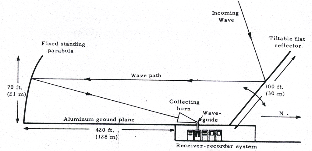
Below is a diagram of the design of the Big Ear radio telescope showing the path that a typical incoming radio wave takes from the source to the flat reflector, then to the paraboloidal reflector, and then into the feed horns and electronics.

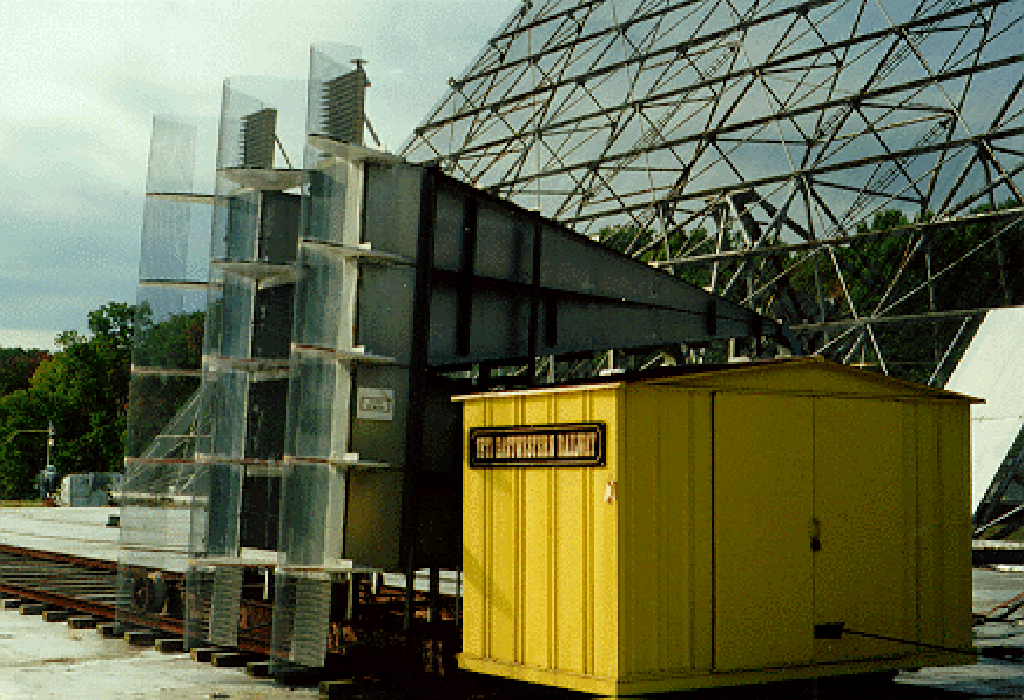
The Big Ear radio telescope was destroyed in 1998 by land developers who purchased the land on which the telescope was located from the Ohio Wesleyan University, Delaware, Ohio, in order to convert a 9-hole golf course into an 18-hole course and to build aproximately 400 houses on the land that they had purchased.

More information can be found about the structures of the "Big Ear", Dr. John D. Kraus (its designer, builder, and Director of the Ohio State University Radio Observatory (OSURO), and the history of discoveries at OSURO by going to the home page of our Big Ear website (at www.bigear.org). [Note. You are already within that website.]

Prior to 1973 the Big Ear radio telescope had been used to measure the location and strength of wideband radio sources; this project was called the Ohio Sky Survey. Most of its operation was in the 21-cm radio band, in which the receiver covered an 8-MHz bandwidth from 1411 to 1419 MHz. [Note: 1 MHz = 1 megahertz = 1,000,000 hertz = 1,000,000 cycles per second.] A total of nearly 20,000 radio sources were measured, about half of which had not been previously measured by any other radio telescope. Many of the Ohio radio sources were observed at other observatories to obtain more accurate positions and optical identifications were made for several of these. Two of these Ohio Sky Survey radio sources were identified as the most distantly-known quasars at that time.

In 1973 the Big Ear radio telescope was converted from measuring the location and strength of wideband radio sources to a similar study of narrowband radio sources. [Note that almost all celestial radio sources (like galaxies, stars, quasars, etc.) are wideband sources (often called continuum sources), generating photons in the radio, optical and even into the X-ray and gamma ray bands. Narrowband sources are almost always purposely generated by intelligent beings (examples include AM, FM, TV and "ham" radio broadcasts, satellite transmissions, and radar).] Due to an unwise decision by the United States Congress in 1972, we lost our funding from the National Science Foundation (NSF) to support the Ohio Sky Survey; this loss of funding also happened to several other universities as well. Eventually, every person employed to work on the Ohio Sky Survey team lost his/her job (except Dr. John Kraus, the Director, who was funded directly by the Ohio State University Department of Electrical Engineering). I was one of those persons. Each of us found employment elsewhere. There was a strong desire to continue to observe with the Big Ear but it had to be in a project that was less human-resources intensive. The systematic search for narrowband signals seemed to be the best way to use that unique radio telescope. My colleague, Dr. Robert S. (Bob) Dixon, the Assistant Director of the radio observatory, convinced Dr. Kraus to convert from wideband observations to narrowband observations. The Big Ear was well designed for a systematic sky survey, as was clearly demonstrated by the success of the Ohio Sky Survey. Also, the combined observing time of all other narrowband observing programs up to that time was very small. Use of the Big Ear would quickly result in our achieving the record for the longest continuously-running survey of narrowband radio emission (indeed, we did achieve that record as described in the "Guinness Book of World Records"), although we didn't purposely set out to achieve that record).

The receiver and associated electronics for the narrowband search were assembled and connected under the leadership of Bob Dixon. Bob and I wrote the software for the IBM 1130 computer used to acquire and analyze the data. Bob wrote most of the initial software to handle the data acquisition and some basic analysis. This was a very large and complicated process involving many main programs and subroutines written in Fortran, where possible, and in assembler language in other cases. I handled the rest of the software, especially that involving some of the more involved analysis of the data (including search strategies). Both of us had other jobs so this was done in our spare time. Bob named this software N50CH.

The IBM 1130 computer running the N50CH program interacted with the receiver to acquire digital intensity values from each of 50 channels (each channel was 10 kHz = 10,000 hertz wide) once each second. Ten of these values were combined to generate one number for each channel and the number for each channel was converted to a single number or letter and printed out (2 seconds were needed for the analysis and printout of each line of information). This entire operation could be handled by the computer with no person present except for starting, stopping, resetting, and restarting the computer.

After the data began to come in regularly, we began a systematic survey of the 100 degrees of declination visible to the radio telescope. (from +64 degrees down to -36 degrees). I took on the task of looking at the computer printout on a regular basis. Gene Mikesell, our mechanical technician at the Big Ear, was trained to stop, reset and restart the IBM 1130 computer every 3 or 4 days. On his way to Columbus for supplies he would deliver the computer printouts to my home.

A few days after the August 15, 1977 detection (probably on August 19), I began my routine review of the computer printout from the multi-day run that began on August 15th. A few pages into the computer printout I was astonished to see the string (sequence) of numbers and characters "6EQUJ5" in channel 2 of the printout. I immediately recognized this as the pattern we would expect to see from a narrowband (i.e., narrow frequency band) radio source of small angular diameter in the sky. In the red pen I was using I immediately highlighted those six characters and wrote the notation "Wow!" in the left margin of the computer printout opposite them. After I completed the review of the rest of the printout (especially to see if the signal returned on subsequent days — it didn't), I contacted John Kraus and Bob Dixon. They were astonished too. Then we began an analysis of what John Kraus began calling the "Wow! signal" (or the "Wow! source"). Analyses have continued even many years afterward as ideas needed to be tested.

The Computer Printout

Let me describe the main features and some of the details about the computer printout. This section will deal with the meaning of the numbers and characters in the printout itself. A later section will deal with other parameters related to the values on the computer printout.

The Page Layout

Below are two important images. Be sure to click on each one to see a larger version.

The first image below (in black & white) is an image of the full page of the computer printout that contains the "Wow!" signal.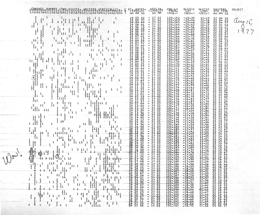

This second image shows only the top part (called the header, also in black & white) of the full page image above. This header shows identifications for each field (type of data in each column or adjacent groups of columns).

Header Columns (Fields): Let me now describe the header (second image) and its relationship to the data placed below the header.

Columns 01 - 50: Each of the first 50 colums shows a 2-digit channel number (from 01 through 50) arranged vertically. Below the header is placed a single character to represent the signal strength for that channel for a given 10-seconds of sampling time, expressed in units of signal-to-noise ratio (S/N ratio = SNR, meaning the signal strength as a multiple of the background noise).

Columns 51 - 53: Column 51 is blank. Column 52 contains CNT arranged vertically. At the time of the "Wow!" signal, this column was not used. Later, it was used to contain a number representing approximately the strength of all 50 channels combined (which we called the "Continuum", hence "CNT"). Column 53 is blank.

Columns 54 - 63: Columns 54 - 63 contain the notation:
RT. ASCEN.
 (1950.0)
 HH MM SS

These columns contain the right ascension (angular distance along the celestial equator – a projection of the earth's equator) measured in time units converted to the epoch of 1950. HH (columns 55 - 56) stands for 2-digit hours (00 - 23), MM (columns 58 - 59) stands for 2-digit minutes (00 - 59), and SS (columns 61 - 62) stands for 2-digit seconds (00 - 59). Column 63 is blank.

Columns 64 - 72: Columns 64 - 72 contain the notation:
 DECLIN.
(1950.0)
   DD MM

These columns contain the declination (angular distance below or above the celestial equator – again, a projection of the earth's equator) converted to the epoch of 1950. Column 64 is blank. Column 65 contains a minus sign when the declination is negative (and is blank for positive declinations). DD (columns 67 - 68) stands for 2-digit degrees (00 - 89, although the Big Ear could observe only in the range from about -36 to + 64 degrees), MM (columns 70 - 71) stands for 2-digit minutes (00 - 59). Column 72 is blank.

Columns 73 - 81: Columns 73 - 81 contain the notation:
2ND LO
 FREQ.
(MHZ.)

These columns contain the frequency at which the 2nd local oscillator (LO) was set. It was adjusted to compensate for the motion of the earth (rotation, revolution, and motion of our solar system around our Milky Way galaxy) about the Galactic Standard of Rest (GSR, essentially, the center of our galaxy). Column 73 is blank. Columns 74 - 80 contain a 6-digit number with 3 decimal places). Column 81 is blank.

Columns 82 - 89: Columns 82 - 89 contain the notation:
GLCTIC
 LAT
(DEG.)

These columns contain the galactic latitude measured in degrees above or below the plane of our galaxy. Column 82 is blank. Columns 83 - 88 contain a signed 4-digit number with 2 decimal places. If the galactic latitude is negative (below the plane of our galaxy) a minus sign appears in column 83; otherwise, that column is blank. Column 89 is blank.

Columns 90 - 96: Columns 90 - 96 contain the notation:
GLCTIC
 LONG
(DEG.)

These columns contain the galactic longitude measured in degrees from a specified starting point; its range is 0.00 to 359.99 (using 2 decimal places). Column 90 is blank. Columns 91 - 95 contain a 4-digit number with 2 decimal places. Column 96 is blank.

Columns 97- 105: Columns 97 - 105 contain the notation:
EASTERN
STD TIME
HH MM SS

These columns contain the Eastern Standard Time (EST) in hours (HH from 00 - 23), minutes (MM from 00 - 59), and seconds (SS from 00 - 59). EST was actually computed from the sidereal (star) time kept by a special clock. EST was always recorded even when EDST (Eastern Daylight Savings Time) was in effect.

Columns 106 - 120: Columns 106 - 120 contain the notation:
OBJECT

There is nothing in these columns. It was planned, but never implemented, to show the names of celestial objects (e.g., known radio sources) near the right ascension and declination being observed.

Note: The line printer for the IBM 1130 computer printed out one line of up to 120 characters simultaneously (in less than 1 second) using a fixed spacing of 10 characters per inch (pica). Hence, there was no capability of using any other spacing or font size. [Note. When standing next to the printer, the printing of one line sounded like "ka-chunk"!]

Now, I will go into more technical detail to describe each of the parameters found on the computer printout. You may look at the following portion of the computer printout that shows about 16 rows of data (about 3 minutes worth). [Click on this image to see a larger one.]

Signal Strength = Intensity

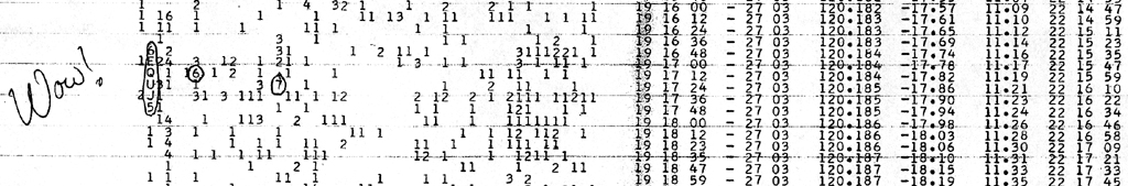
Each row of the computer printout represents the results of the data collected during approximately 12 seconds of sidereal (star or celestial) time. 10 seconds were used to obtain the average intensity for each of 50 channels and approximately 2 seconds were used by the computer to process the data and analyze it for possible interesting phenomena. During each 10-second period of data acquisition, one intensity was obtained each second for each channel and then the 10 values obtained over the 10 seconds were averaged for each channel. The left hand half of each row on the computer printout shows the intensity for each of the 50 channels with channel 1 leftmost and channel 50 rightmost. Due to limitations of space on the computer printout, Bob Dixon decided to use a single character to represent each intensity. The average intensity over the 10-second integration period for each channel was converted into an integer number or character by the following 5-step process:

• Step 1: the average intensity of 6 integration periods (1/6 of the current value plus 5/6 of the previous value) was subtracted out to remove the baseline intensity;
• Step 2: the remainder was divided by the standard deviation computed over 60 integration periods (1/60 of the current value plus 59/60 of the previous value) ( note that the standard deviation is equivalent to the noise);
• Step 3: the number in Step 1 was divided by the number in Step 2, which gave the signal to noise ratio (S/N);
• Step 4: the integer portion of this S/N ratio was taken (i.e., the value was "truncated" to an integer); and
• Step 5: the integer was printed out as follows: an integer value of zero was "printed" out as a blank, the integer values from 1 through 9 were printed directly, and integer values from 10 through 35 were printed out as the upper case letters A through Z, respectively (e.g., the integer value 10 was printed out as A, the integer value 11 was printed out as B, etc.).

Note that the calculations in Steps 1 and 2 (for the baseline intensity and the standard deviation) were omitted (i.e., keeping the previous values) when the signal strength exceeded a predetermined threshold.

The signal-strength sequence "6EQUJ5" in channel 2 of the computer printout thus represents the following sequence of signal-to-noise ratios (S/N):
6 --> (6 up to 7)
E --> (14 up to 15)
Q --> (26 up to 27)
U --> (30 up to 31)
J --> (19 up to 20)
5 --> (5 up to 6)

The strongest intensity received ("U") means that the signal was 30.5 +/- 0.5 times stronger than the background noise (note that the notation "+/-" means "plus or minus" representing a range of values, in this case from 30.5 - 0.5 = 30.0 up to 30.5 + 0.5 = 31.0). Most of this background noise is generated within the receiver itself, but some noise comes from the trees, grass and other surroundings, and some from the celestial sky (the remnant of the "Big Bang" that is estimated to have occurred about 13.7 billion years ago).

Here is a plot made by Dr. Kraus of the signal strength vs. uncorrected right ascension (i.e., as read from the computer printout). He has hand drawn a smooth curve to fit the 6 data points. He has indicated that the half-power beam width (HPBW) of this signal was 37 seconds (of celestial time or right ascension). The HPBW means the length of time that it took the signal to rise from a power (signal-strength) level of 50% of the maximum to the maximum and back down to the 50% level. Some persons have misunderstood this value of 37 seconds by declaring that the "Wow!" signal lasted only 37 seconds. That is incorrect! The signal lasted about 72 seconds, because we had 6 data points (6EQUJ5) with a separation between data successive points of 12 seconds (hence, 6 times 12 = 72).

Right Ascension and Declination

The next two groups of numbers on the computer printout (just to the right of the center of the row) are the right ascension and declination converted to epoch 1950.

Right ascension is analogous to longitude on the earth's surface. It is measured in either degrees (0 to up but not including 360) or in hours (h), minutes (m), and seconds (s) (00h00m00s up to but not including 24h00m00s). The starting point (0 degrees = 0 hours) is currently in the constellation of Pisces but is moving slowly although constantly (it takes about 26,000 years to make a complete circuit; the major component of this motion is called the "precession of the equinoxes"). Because of this precession and other related but smaller effects, astronomers convert the observed positions at any one instant into one appropriate for a convenient point in time so that locations can be more easily compared. The epoch (point in time) of 1950 was most commonly used during the middle to late part of the 20th century. Nowadays, the year 2000 is the epoch most likely used.

Declination is the angular distance above or below the projection of the earth's equator onto the celestial sky (and is analogous to latitude on the earth's surface). Its range of values goes from -90 degrees (at the south celestial pole) through zero (on the celestial equator) and then up to +90 degrees (at the north celestial pole). The Big Ear radio telescope could observe in the 100-degree range of declination from approximately -36 degrees to approximately +64 degrees.

For the strongest Wow! data point, the epoch 1950 right ascension shown on the computer printout was: 19h17m24s, while the corresponding declination was: -27 degrees (d) and 3 minutes (m) of arc (-27d03m). This puts the source in the direction of the constellation Sagittarius. [Note, however, that the constellation name gives just the general direction and provides negligible useful information to an astronomer (who usually need to have a very precise position (right ascension, declination, and epoch)).]

It turns out that prior to the occurrence of the Wow! signal, I made a mistake in the computer programming in dealing with the correction of the R. A. coordinate for the offset of the positive horn. I added the correction rather than subtracting it as I should have. I corrected this error when it was discovered, which, unfortunately, was after the Wow! source was detected. Later in this article, I will compute the corrected value for R.A.

2nd L.O. Frequency (and the Corresponding Frequency of Observation)

The computer printout shows a 2nd L.O. (local oscillator) frequency of 120.185 MHz for the strongest datapoint (the one showing an intensity represented by the letter "U"; the 4th of 6 data points). What is meant by that frequency?

Before I answer that question, let me show a block diagram of the receiver, courtesy of Dr. Robert S. (Bob) Dixon and taken from a preprint of an article by him entitled "The Ohio SETI Program — The First Decade".

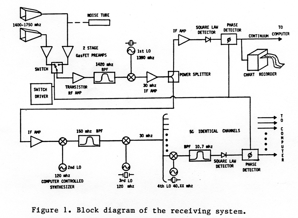
[Be advised that the notation "mhz" used on this diagram has been replaced by "MHz" in recent years. "MHz" means "megaHertz", where "mega" refers to one million and "Hertz" refers to frequency measured in cycles per second. For example, 1400 MHz refers to a frequency of 1400 millions of cycles per second.]

During the planning stages of putting the receiver together, Bob Dixon decided that observations would be conducted in a frequency band around 1420.4056 MHz (MHz means megahertz = millions of Hertz = millions of cycles per second), the frequency of the neutral hydrogen line for the case when there is no line-of-sight motion between our receiver and the source of the neutral hydrogen line (transmitter). Since hydrogen is the most abundant element in the universe, there is good logic in guessing that an intelligent civilization within our Milky Way galaxy desirous of attracting attention to itself might broadcast a strong narrowband beacon signal at or near the frequency of the neutral hydrogen line. Bob surmised further that such a civilization might change its transmitter frequency in such a way as to remove the effect of the Doppler shift of frequencies that occurs when its transmitter is either moving towards or moving away from the receiver. If the transmitter frequency were adjusted to compensate for its motion with respect to the center of our galaxy (called the "local standard of rest" = LSR) and if our receiver frequency were separately adjusted to compensate for its (and our) motion with respect to the same LSR, then we should see their beacon signal right in the middle of our receiver channels if it were strong enough and if it were in our beam.

The 50-channel receiver we had available to us was built by the National Radio Astronomy Observatory (NRAO) in Green Bank, West Virginia. It was designed to operate so that the boundary between channel 25 and channel 26 (i.e., exactly halfway through the 50 channels) occurred at 150 MHz. At the same time, we had an intermediate-frequency (I.F.) amplifier that operated in a band centered at 30 MHz, and we needed to use that amplifier as a part of the chain of electronics to boost the very small signal so that the subsequent electronics (including an analog-to-digital (A/D) converter) would have sufficient voltages that could be converted into numbers to be recorded and analyzed by the computer. Thus, for the case when there is no line-of-sight motion between us and our LSR, we needed to have the neutral hydrogen line frequency of 1420.4056 MHz be eventually converted into 150 MHz with amplification at 30 MHz occurring in between.

The plan was as follows.

• Step 1: Mix a 1st local oscillator (1st L.O.) signal at 1450.4056 MHz with the weak desired neutral hydrogen line signal at 1420.4056 MHz to yield an output signal at 30 MHz;
• Step 2: Amplify this 30 MHz signal by the I.F. (intermediate frequency) amplifier;
• Step 3: Mix a 2nd local oscillator (2nd L.O.) signal at 120 MHz with the output of the 30 MHz signal to obtain a signal at 150 MHz; and
• Step 4: Send that 150 MHz signal into the 50-channel receiver. Note that the 2nd L.O. could be varied around 120 MHz to adjust the observing frequency at the center of the 50 channels to our LSR.

There was a minor glitch to the above plans, and it occurred in Step 1 above. It was discovered that the 1st L.O. was set by the manufacturer to 1450.5056 MHz (or 0.1000 MHz above the desired frequency of 1450.4056 MHz). In order to compensate for that offset of 0.1000 MHz, the 2nd L.O. would have to be set 0.1000 MHz lower than planned (e.g., at 119.9000 MHz instead of 120.0000 MHz).

The bottom line to the above discussion is that the difference between the 2nd L.O. frequency and 119.9 MHz is added to 1420.4056 MHz to obtain the frequency of observation at the boundary between channel 25 and channel 26. Since each channel was 0.0100 MHz (10 kHz = 10 kilohertz = 10,000 Hz) wide, then 0.0100 MHz would have to be subtracted off for each channel below the channel 25-26 boundary.

The computer printout shows a 2nd L.O. frequency of 120.185 MHz at the time of the strongest of the 6 data points. Subtracting 119.9 MHz yields a difference of 0.285 MHz and adding this to 1420.4056 MHz yields a frequency of observation at the channel 25-26 boundary of 1420.6906 MHz. It is necessary to move down 23.5 channels to get to the middle of channel 2; thus we must subtract 0.235 MHz from the center frequency to obtain the observing frequency for the center of channel 2. That value is: 1420.4556 MHz.

In conclusion, we can say that the frequency of observation of the Wow! source was 1420.4556 +/- 0.005 MHz (note that the error of +/- 0.005 MHz represents one half of the width of channel 2, or any other channel).

Galactic Latitude and Longitude

The next two groups of numbers on the computer printout are the galactic latitude and galactic longitude converted to epoch 1950.

Galactic latitude is the angular distance above or below the plane of our galaxy. It's range of values goes from -90 degrees (at the south galactic pole) through zero (in the plane of our galaxy) up to +90 degrees (at the north galactic pole).

Galactic longitude is analagous to longitude on the earth's surface. It is measured in degrees (0 up to but not including 360) relative to a defined starting point very near the direction of the center of our galaxy.

Precession of the equinoxes, among other apparent motions, affects the computed galactic coordinates in a manner similar to the way right ascension and declination are affected.

For the strongest data point of Wow!, the computed epoch 1950 galactic latitude was -17.86 degrees and the corresponding galactic longitude was 11.21 degrees. Thus, the Wow! source direction was about 18 degrees below the plane of our Milky Way galaxy and a total of about 21 degrees from the direction of the galactic center.

Eastern Standard Time

The computer was reading a sidereal (star-time) clock to keep track of time. Eastern Standard Time (EST) was computed from the sidereal time. Sidereal time covers 24 of its hours in about 23 hours 56 minutes and 4 seconds of our standard time. By the way, even though it was August for these observations and, in Ohio, our civil time was Eastern Daylight Savings Time (1 hour ahead of EST), we computed and printed out EST to be consistent year around. Note that the Wow! source was observed around 22:16:34 EST (about 10:16 p.m. EST or 11:16 p.m. EDT). No one was at the telescope at that time. The receiver and computer were doing their jobs unattended.

Analyses of Wow! to Correct Errors

Even though anyone can read the values in the computer printout and draw conclusions from them, there is information not given in the computer printout that must be taken into account before drawing certain conclusions. That additional information will be provided in this section while describing some of the analyses done by my colleagues and by me.

Source Location

Effect of Dual-Horn Feed System

The Big Ear used a dual-horn feed system. A "feed horn" is a large funnel-shaped metal structure (we used aluminum) located between the flat and curved reflectors designed to collect the energy focussed by the curved paraboloidal reflector located at the south end of the radio telescope. The two feed horns were located side by side in the focal region of the paraboloid 420 feet north of the vertex of the paraboloid. The westernmost feed horn was located about 8.79 feet west of the focal point. The easternmost feed horn was located about 4.10 feet west of the focal point. Thus, the two horns were separated by about 4.69 feet along an east-west line. The receiver was configured as a Dicke switching receiver, switching from one horn to the other horn and back again 79 times per second (79 Hz). The receiver used a synchronous detector that measured the difference between the signals coming from the two horns such that the signal coming from the westernmost horn (the west horn) was subtracted from the signal coming from the easternmost horn (the east horn). This difference signal was then amplified, fed into the 50-channel detector, each channel was digitized, and the digital data was fed to the computer for analysis. The west horn was also called the negative horn while the east horn was called the positive horn. Thus, the Dicke switching receiver subtracted the negative horn signal from the positive horn signal. As the earth's rotation swung the two beams across the celestial sky, a signal (with positive energy) from a radio source was first seen by the west (negative) horn and generated an inverted bell-curve-like shape on the chart recorder. Within a minute or so after the negative horn response was essentially complete (i.e., showed little energy from the source), the same radio source began to be scanned by the east (positive) horn and a non-inverted (right-side up) bell-curve-like shape on the chart recorder was generated. Thus, for a strong radio source of small angular diameter like a distant galaxy or quasar, we see a negative (inverted) beam response followed by a positive beam response shortly thereafter. However, this was not the case for the Wow! source.

The computer printout for Wow! shows only one detection instead of the two detections expected with the dual-horn system. At the time of this signal (August 1977) the computer was not programmed to identify whether the observed output was negative (from the negative horn) or positive (from the positive horn). [Note. Later, the computer was reprogrammed to overprint a minus sign on any printed negative intensity (except a blank representing a signal-to-noise ratio of 0 up to 1).] Unfortunately, this lack of knowledge about which horn the Wow! signal entered leads to an ambiguity in the calculated source position. Below the two possible right ascensions are derived.

It would be a fair question to ask if the analog chart record wouldn't resolve the discrepancy. Nice thought but no such luck. An analog chart record was generated for the continuum (wideband) receiver. That is, while the 50-channel receiver was operating, a separate wideband (8 MHz wide) receiver was also operating. It was called the "continuum receiver" because continuum radio sources (like galaxies, quasars, nebulae, and stars) generate radio waves over the entire radio spectrum (as well as in the optical spectrum plus the rest of the electromagnetic spectrum). Its output was digitized and available for analysis, but in addition, its output (before digitization) was recorded on an analog stripchart recorder. Although this continuum receiver easily shows continuum sources with flux densities of about 0.5 janskys or more (where the radio emission covers the entire radio band), a narrowband radio source like the Wow! source would not be (and was not) detected. Let me illustrate.

Suppose a narrowband radio source generated enough energy in a 10 kHz (0.01 MHz) band to be equivalent to a flux density of 50 janskys (but only in that narrow band). What would be seen with a receiver 8 MHz wide. The averaging process that would automatically occur (and is unavoidable) would cause the continuum receiver to see a signal only 0.01/8 (or 1/800) of the strength seen in the narrowband channel. In other words, the hypothetical 50 jansky narrowband source would appear as a 50/800 = 0.0625 jansky wideband source, and that would be undetectable. That is what happened to the Wow! source. Since it appeared in only one 10 kHz channel, it contained little or no energy in other channels. Hence, the average of strong energy in one narrowband channel with negligible energy in the equivalent of 799 other channels yields a very low average energy, so low that it is buried in the noise of the narrowband channel.

Determination of Corrected R.A. Assuming Positive Horn Received Signal

Since there is an ambiguity in the right ascension (R.A.) because we do not know in which beam the source was observed, what are the two possible positions?

The computer printout shows the epoch 1950 right ascension (R.A.) of the highest data point as 19 hours 17 minutes and 24 seconds of time (or 19h17m24s, for short). The corresponding declination was -27 degrees and 3 minutes of arc (or -27d03m, for short). It is necessary to understand that the printed R.A. is computed under the assumption that the source was seen in the positive (east) beam and that each R.A. represents the converted epoch 1950 value at the end of each 10-second integration (averaging) period. Also remember that I had made an error in applying the horn offset (horn squint) in R.A. so this error must be corrected.

19h17m24s represents the end of the 10-second integration period that yielded an intensity (signal-to-noise ratio = S/N) of 30 (the letter "U"). However, it is better to state the R.A. at the center of each 10-second integration interval because it is more representative of the interval. Therefore, subtracting 5 seconds from the computer printout positions yields 19h17m19s for the R.A. of the largest data value applying the offset to the center of the integration interval.

Let's now deal with correcting the misapplication of the horn squint (offset) in R.A. The computer acquisition and analysis program (N50CH) had built into it a horn squint in R.A. of minus 138/cosine(declination). This number means that at the equator (declination = 0) the R.A. horn squint for the positive horn was minus 138 seconds of R.A. At the declination of Wow! (-27d03m), this horn squint would compute to minus 154.95 seconds of R.A. According to Debbie Cree, a student who did a project and wrote a report in 1980 on the Big Ear under the supervision of John Kraus, the positive horn was 4.10 feet west of the focus; hence, the Wow! source would have achieved its maximum intensity in that positive horn 154.95 seconds of R.A. before it would have if that positive horn had been located at the focus. Thus, the calculated R.A. would be too small by that amount. I should have subtracted the negative horn squint in order to create a larger R.A. Instead, I inadvertently added it. Thus, in order to correct for this error, simply double the value of 154.95s and add it to the printed R.A. Since 2 * 154.95s = 309.90s = 5m9.90s (or approximately 5m10s), we do the following calculations to the printed R.A. for the 6 data points.

In the table below the first column presents the character used for the intensity, the second column shows the original (incorrect) right ascension (epoch 1950) on the computer printout, the third column shows the corrected epoch 1950 R.A. for the end of the integration interval (adding 5m10s to the original R.A.), and the last column shows the corrected epoch 1950 R.A. for the middle of the integration interval (subtracting 5s from the third-column results).

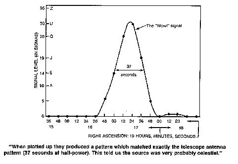
From the above table, using the middle of the interval containing the largest data point, we have the R.A. of the Wow! source near 19h22m29s under the assumption that it came in the positive horn. A better position can be obtained if one fits the antenna pattern to the Wow! data and determines the R.A. where the peak of that pattern occurs. I did such an analysis. I fit two different mathematical functions (as approximations to the antenna pattern) to the Wow! data. One was the well-known bell curve (also know as a Gaussian curve or normal curve). The second function was of the form (sin(x)/x)^2, where the notation "^2" means raising to the 2nd power (squaring). These two functions are very similar from the peak down to somewhat below half amplitude. Well below half amplitude the second function displays multiple secondary peaks and valleys while the Gaussian steadily drops toward a zero value. The second function thus looks closer to what a strong source might look like (i.e., having sidelobes). However, the Wow! source was not strong enough to display sidelobes, so either function used as an approximation to the real antenna pattern is a suitable fit.

In fitting the Wow! data to each of the two functions, each of the six intensity values was increased by 0.5 to account for the truncation error (in which the fractional portion is discarded and only the integer portion is kept; remember this was done because there was space on the computer printout for only 1 character to represent the signal strength for each channel). That is, since the first intensity of 6 could have been anywhere in the range from 6.0 up to but not including 7, the value of 6 + 0.5 = 6.5 is the best estimate of the actual value. Similarly, the value "U" representing a S/N of 30 is really some value at or above 30.0 but below 31; hence I used 30 + 0.5 = 30.5 for the best estimate of the untruncated value. Thus, the sequence "6EQUJ5" represented the signal-to-noise (S/N) intensities: 6.5, 14.5, 26.5, 30.5, 19.5, and 5.5, respectively; an uncertainty of +/- 0.5 must be assigned to account for these truncation errors. [Note that the system noise itself creates an error of 1.0 (at the 1-sigma level by definition (which corresponds to a 68.26% confidence level) or an error of 2.0 at a 95.44% confidence level).]

The 5-second subtraction of R.A. for each data point, as described above, was also used, but the 5m9.9s corrected for the misapplication of the horn squint was not used.. The best fit curves for the two functions yielded the following positive horn R.A. at the peak:

Model 1: (Gaussian): 19h17m14.82s

Model 2: ((sin(x)/x)^2): 19h17m14.66s

Applying the 5m9.9s correction for the misapplication of the horn squint yields the following corrected values:

Model 1 (Gaussian): 19h22m24.72s

Model 2: ((sin(x)/x)^2): 19h22m24.56s

Thus, the two models agree within 0.16 seconds of time. Using an average of these two models yields a corrected R.A. of the Wow! source under the positive horn assumption of 19h22m24.64s

Note that the corrected value of 19h22m24.64s is 4.36s smaller than the corrected R. A. of the 4th data point (the one with the largest intensity). This makes sense when you view a plot of the 6 data point intensities vs. time. The peak of the best-fit curve must be in between the 3rd and 4th data points but closer to the 4th data point.

By the way, a calculation of the residuals for each function showed that the Gaussian was a slightly better fit than the (sin(x)/x)^2 model, although the differences were small (in fact, for 3 of the 6 data values the Gaussian had the smaller residuals while the reverse occurred for the other 3 of 6 data values).

Determination of Corrected R.A. Assuming Negative Horn Received Signal

Now let's determine what the R.A. would have been under the assumption that the signal came in the negative horn. In the 1980 report by Debbie Cree, she quotes the location of the east (positive) horn as 4.10 feet west of the focus, and the location of the west (negative) horn as 8.79 feet west of the focus. Thus, the difference in distance between the two horns is 4.69 feet (along an east-west line). The focal length of the paraboloidal reflector is 420 feet. The horn center, the focal point and the vertex of the paraboloid, all projected onto the ground plane, form a right triangle. The focal length (420 feet) is the long leg, the horn offset is the short leg at a right angle to the long leg, and the hypotenuse is the line from the horn to the vertex. For each horn, we desire to know the angle opposite the short leg. The difference between those two angles equals the angle in the sky separating the peaks of the two beams.

First, lets compute the two angles, initially in arcminutes, then in seconds of time at the equator, and finally, in seconds of time at the declination of the Wow! source (-27.05 degrees). Call the two angles theta_pos and theta_neg. Note that "pi" = 3.141592654 (approximately) in the formulas below.

Negative horn at 8.79 feet: theta_neg = (180/pi)*60*arctan(8.79/420) = 71.9366 arcminutes.

Positive horn at 4.10 feet: theta_pos = (180/pi)*60*arctan(4.10/420) = 33.5579 arcminutes.

Note that the factor arctan(offset/focal length) yields the angle in radians, the factor (180/pi) converts the radians into degrees, and the factor 60 converts degrees into minutes of arc (i.e., arcminutes). Expressing these results in seconds of R.A. at the equator by multiplying by 4 yields:

Negative horn: theta_neg = 287.75 seconds = 4 minutes 47.75 seconds.

Positive horn: theta_pos = 134.23 seconds = 2 minutes 14.23 seconds.

To convert an angle into time or R.A. units away from the equator, one must divide by the cosine of the declination. Using cos(-27.05 degrees) = 0.89061, we have the following results for the Wow! source:

Negative horn: theta_neg = 323.09 seconds = 5 minutes 23.09 seconds.

Positive horn: theta_pos = 150.72 seconds = 2 minutes 30.72 seconds.

Now we compute the difference between these last two results to obtain 172.37 seconds = 2 minutes 52.37 seconds as the R.A. difference between the peaks of the positive and negative horns for the Wow! source. Because the negative beam goes through a given radio source before the positive beam does, and because the calculation in the previous subsection computed the R.A. under the assumption that the source came through the positive beam, it is necessary to add this 172.37 second difference to obtain the R.A. for the assumption of a negative beam detection. Using the best fit value from the two mathematical functions shown above, that value is:

Negative beam R.A. for Wow! = 19h22m24.64s + 00h02m52.37s = 19h25m17.01s.

Estimated Errors in Computed R. A. and Declination Values

Before estimating errors in the computed R. A. and declination, let's restate those epoch 1950 values:

R.A. (positive horn assumption): 19h22m24.64s

R.A. (negative horn assumption): 19h25m17.01s

Declination: -27d03m

Let's deal with declination first, because it is the simplest. The horn offset in declination (for each horn) was 1 degree (or 60 arcminutes), as accurately as we could measure it; this corresponded to the centers of the horns being about 7 1/3 feet above ground. A horn above ground makes less of an angle with respect to a horizontal line from the center of the paraboloid to the point on the flat at the same height above ground, and also a smaller angle of incidence to the flat reflector than would a horn located at ground level. Thus, the effect of the horn squint of 1 degree in declination means that 1 degree needed to be subtracted from the declination setting (-26d00m for the Wow! source) to obtain the squint-corrected declination of -27d00m for the time of the observation. Applying the precession and other corrections to convert to epoch 1950 yielded the declination of -27d03m, the same as was shown on the computer printout.

I estimate the error in the declination squint to be about 1 arcminute. However, there is a much larger source of error. Since Wow! was observed only one time (at only one declination, of course), there was (and is) no way to estimate the declination by comparing the source strength at other declinations. Normally, as was routinely the case with the continuum sources in the Ohio Sky Survey, observations at 20 arcminutes above and 20 arcminutes below the declination that gave the largest intensity permitted a calculation of the declination where the peak intensity would have been observed. [Note that the half-power beamwidth = HPBW was 40 arcminutes; choosing one half of the HPBW (or 20 arcminutes) to be the standard increment in moving the telescope in declination yielded the fastest possible survey while still maintaining the ability to accurately determine the declination of sources visible at two or more adjacent declinations.] So for the Wow! source, seen at only one declination, it is reasonable to assign an uncertainty (error) in declination position of 20 arcminutes. By the way, since the squint error and the error due to seeing the source at only one declination are independent, the statistical procedure of taking the square root of the sum of the squares of the independent errors yields: square root (20*20 + 1*1) = square root (401) = 20.025 arcminutes. Since this is so close to 20 and since the component error of 20 arcminutes itself was an estimate, it is OK to state that the error in declination is 20 arcminutes.

Now let's deal with the R.A. errors. First let's consider the error in the squint of the two horns. In the above calculations I used the horn squint for the positive horn as -138/cosine(declination). This value was based on many measurements of sources with known R. A. in the Ohio Sky Survey and was appropriate for the Wow! source measurements because the positive horn was not moved between the period of the Ohio Sky Survey and the occurrence of the Wow! signal.

However, about three years after the Wow! source occurrence, Debbie Cree measured the physical location of the positive and negative horns as 8.79 feet west and 4.10 feet west of the focus, respectively. As far as we can remember, the positive horn was not moved during those three years between the Wow! source occurrence and Debbie Cree's measurements. However, her measurements do yield a slightly different positive horn squint in R.A.

Recall from above, I calculated that the 4.10 foot offset of the positive horn would yield a R.A. squint of -134.23s at the equator or -150.72s at the Wow! source declination. Compare these with the adopted value (from the Ohio Sky Survey) of -138s at the equator or -154.95s at the Wow! source declination. The difference between -150.72s and -154.95s is 4.23s. Having applied the R.A. squint in the wrong direction, I had to double the squint and subtract to correct for the error. If I were to use Debbie Cree's measurements and the squint derived from those measurements, I would have to subtract twice 4.23s from my previously stated R.A.s (both positive horn and negative horn) for the Wow! source. Rather than adopt Debbie Cree's measurements and the assumption that the focus is where she thought it was, I choose to use the -138/cosine(declination) calculation but assign any differences into the error. Thus, one component of the error in R.A. will be taken as 2*4.23s = 8.46s.

A second component of error occurs with uncertainty in the sidereal clock read by the computer and used as the basis for all position measurements (except declination) and for Eastern Standard Time (which was computed from sidereal time). The clock that was in use during the SETI program had been used throughout the Ohio Sky Survey where it had kept good time. However, as it grew older, it became less reliable. Occasionally, we would notice that it was off by as much as 2 seconds of time (very large for a precision astronomical clock). Thus, I will assign an error of 2s for this second error.

A third component of error is the measurement error due to the size of the beam in R. A. At the equator the beam size (half-power beamwidth = HPBW) is 8 arcminutes. At the equator this converts to 32 seconds of R.A., and at the Wow! declination it converts to 35.93s. I estimate that a measurement error of 1 arcminute could arise for a source with the strength of Wow!. Converting this into seconds of R.A. at Wow!'s declination we have a value for this third error of 4.49s.

Thus, assigning independent errors of 8.46s, 2s, and 4.49s yields a combined error of: square root (8.46*8.46 + 2*2 + 4.49*4.49) = 9.78s. Because of the various uncertainties, I will call the total error 10s and will round all R.A. values to the nearest second.

Summarizing, we have the corrected and final R.A.s and declination for the Wow! source with their estimated errors as follows:

R.A. (positive horn): 19h22m25s +/- 10s
R.A. (negative horn): 19h25m17s +/- 10s
Declination: -27d03m +/- 20m

Conversion of Right Ascension and Declination to Epoch 2000

The two values of right ascension (for the two horns) and the value of declination for the Wow! signal shown at the end of the last section were based on epoch 1950. Since we are past the year 2000, most astronomers are now reporting the celestial coordinates of objects using the epoch 2000. Thus, I will convert the above coordinates into epoch 2000 values.

Because of the size of the errors (+/- 10s in right ascension and +/- 20m in declination), I will simplify the computation to consider only precession taking into account only the first order terms. Nutation and aberration plus higher-order terms of precession would need to be taken into account if our precision were better than 1 second of time or a few seconds of arc.

The expressions I will use are as follows:
delta_R.A. = m + n*sin(R.A.)*tan(dec.)
delta_dec = n*cos(R.A.)
m = 3.07234 +0.00186*T
n = 20.0468 - 0.0085*T
T = 0.75

Delta_R.A. is the expression for the additive change in right ascension for one year of precession, measured in seconds of time (or seconds of R.A.). Delta_dec is the expression for the additive change in declination for one year of precession, measured in seconds of arc. Trig functions of sine (sin), cosine (cos) and tangent (tan) are used. The parameters "m" (measured in seconds of R.A.) and "n" (measured in seconds of arc) are computed as linear functions of T, the number of tropical centuries from the year 1900 involved in the change. Because we are going from epoch 1950 to epoch 2000, I will use the average values of m and n for the average epoch of 1975 (which is 0.75 tropical century from 1900).

Doing the computations for m and n, we have:
m = 3.073735 seconds of R.A., and
n = 20.040425 arcseconds = 1.3360283 seconds of R.A. (the latter is obtained by dividing the former by 15, since, at the equator, 15 arcseconds = 1 second of R.A.).

Now computing delta_R.A. we have for the two horns:
delta_R.A. (positive horn) = 3.7123 seconds of R.A.
delta_R.A. (negative horn) = 3.70925 seconds of R.A.

Since delta_dec involves right ascension, I will compute delta_dec for both the positive horn and the negative horn. The results are:
delta_dec (positive horn) = 7.05242 seconds of arc
delta_dec (negative horn) = 7.28650 seconds of arc.

Now multiplying each of these by 50 years, the total precessional corrections to be added to R.A. and declination, respectively, are:

Positive horn:
R.A. correction = 185.615s = 3m5.62s (approximately 3m6s);
declination correction = 352.62 arcseconds = 5.877 arcminutes (approximately 6 arcminutes).

Negative horn:
R.A. correction = 185.463s = 3m5.46s (approximately 3m5s);
declination correction = 364.325 arcseconds = 6.072 arcminutes (approximately 6 arcminutes).

Now adding these corrections to the epoch 1950 positions, using the approximate values because of the large error bars, we have as the epoch 2000 coordinates of Wow! the following:

R.A. (positive horn): 19h22m25s +/- 10s +3m6s = 19h25m31s +/- 10s
R.A. (negative horn): 19h25m17s +/- 10s +3m5s = 19h28m22s +/- 10s
Declination: -27d03m +/- 20m +6m = -26d57m +/- 20m

Galactic Latitude and Galactic Longitude

Since the computed R.A. for the positive horn on the computer printout was wrong, and since I have obtained a corrected value for it as well as for the R. A. for the negative horn, the printed galactic coordinates need to be recomputed. I will do this by simply computing differences.

Looking at the computer printout, I record below the galactic latitude and galactic longitude for the two printed rows having R.A.s of 19h13m00s and 19h18m00s, respectively.

Thus, when R.A. increases by 5m (300s), the galactic latitude decreases by 1.03d (61.8m) and the galactic longitude increases by 0.44d (26.4m). Applying these rates linearly for both R.A. positions and for the +/- 10s error estimates (OK for the small changes in R.A.), the corrected and deduced R.A.s for the two horns yield corrected galactic latitudes and longitudes and estimated errors as shown in the table below.

Eastern Standard Time

Since Eastern Standard Time (EST) was computed directly from the date and the sidereal time (read from the sidereal clock), the error in applying the horn squint in R.A. did not affect EST. However, from the best fit analysis referred to above, the computed peak of the Wow! source occurred 4.36s prior to the time of the 4th data point. Also, the EST on the printout referred to the end of the integration interval rather than the middle of that interval. Thus, we should subtract 4.36s to account for the peak of the source and subtract another 5s to shift from the end to the middle of the integration interval. Doing so results in the following EST for the peak of the Wow! source: 22h16m10s - 4.36s -5s = 22h16m00.64s = approximately 22h16m01s (or 10:16:01 pm). Since Eastern Daylight Savings Time (EDT) was in effect at the time, the Wow! source peak occurred at about 11:16:01 pm EDT.

Frequency of Observation

In the above subsection entitled "2nd L.O. Frequency (and Frequency of Observation)" under the section "Computer Printout", the frequency band in which Wow! occurred was calculated. Since the calculation of the observing frequency (specifically, the setting of the 2nd L.O. frequency) was based on the date and the sidereal clock, there is no need to redo the calculation I did earlier; that is, the R.A. horn squint error had no effect on the calculation of the observing frequency.

Vast Conclusions from "Half-Vast" Data

As an aside, the above discussions and calculations should provide ample evidence that a person not familiar with all of the special knowledge about a particular instrument and its related computer software should not try to draw too many conclusions from printed data. Such data typically contains certain assumptions about the equipment not necessarily known to outsiders.

Other Analyses

WOWFIT

In the above subsection entitled "Determination of Corrected R.A. Assuming Positive Horn Received Signal" under the section entitled "Analyses of Wow! to Correct Errors", reference was made to fitting two mathematical models (Gaussian and (sin(x)/x)^2) to the Wow! data. I gave each of several variations of this fitting the general name WOWFIT. Not only was the position of the peak found, also determined were: the half-power beamwidth (HPBW), the peak intensity, and a measure of the goodness of fit called the "error sum of squares" (typically denoted in statistics by the notation "SSE").

In one variation of WOWFIT called WOWFIT6P, I allowed each of the 6 data points to be adjusted either up or down by 1 unit or else remain unchanged. That meant 3 possible states for each of the 6 data points. This generated 3*3*3*3*3*3 = 3^6 = 729 cases for each of the two models. Before making any adjustment to a data point, each of the original data points had been incremented by 0.5 to account for the truncation error caused by chopping off (truncating) the actual intensity value to the integer portion so that a single character could be used on the computer printout for each intensity for each channel. An iteration (i.e., trial and error) procedure was used to obtain the best-fit curve to the adjusted data because three parameters had to be determined (location of the peak, amplitude (intensity) of the peak, and HPBW), and a direct solution was not possible. Typically, it took between 4 and 7 iterations to zero in on a solution.

The first case considered was the one where none of the six data points was adjusted (except for the truncation error adjustment applied in all cases to all six data points). For this case, the Gaussian gave a slightly better fit (SSE = 7.525) than the (sin(x)/x)^2 model (SSE= 10.542). The results of this case for the Gaussian are as follows:

Location = 14.82s which corresponds to a corrected epoch 1950 R. A. assuming the positive horn of 19h22m24.72s;
Amplitude = 30.76 (meaning the signal-to-noise ratio at the peak (S/N) was 30.76); and
HPBW = 38.62s (at the declination of Wow! (-27d03m); converting this to the equator (declination = 0d) yields a HPBW = 34.395s = 8.599 arcminutes.

Location = 14.28s;
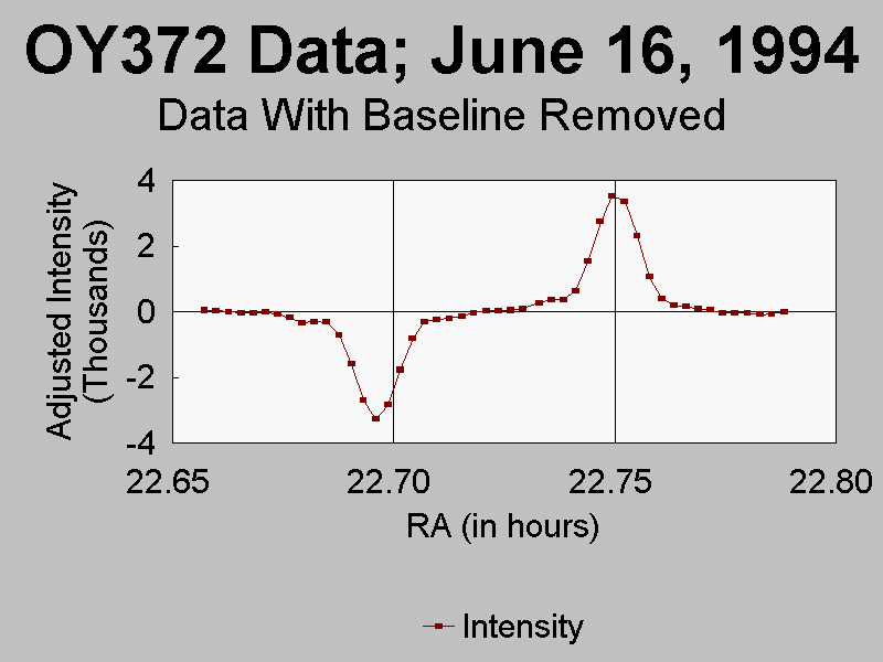
Amplitude = 30.53; and
HPBW = 39.07s.

I should note that the best fit using the (sin(x)/x)^2 model was somewhat worse (SSE = 1.451) than the best fit with a Gaussian (SSE = 0.321).

In Which Horn Did Wow! Enter? Use of OY372 Data for Antenna Pattern Fits

Data from June 16, 1994 on the moderately strong point source OY372 (flux density of 11.53 janskys (Jy)) were provided to me by Russ Childers (who was the Chief Observer at the Big Ear for many years and who is continuing in that role for our Argus array at NAAPO (North American AstroPhysical Observatory in Columbus, Ohio). Russ had been conducting a narrowband survey (which he called LOBES) and a concurrent repeat of the wideband Ohio Sky Survey). [Note. 1 jansky (Jy) = 10 raised to the -26th power watts per square meter per hertz = 10^-26 W m^-2 Hz^-1; this measn that 1 jansjky represents 1 one hundredth of a trillionth of a trillionth of a watt of energy falling on one square meter of collecting area in a one hertz bandwidth.]

The image to the left shows the response of the Big Ear radio telescope to the moderately strong point source OY372. It shows the negative response (the beam of the negative horn crossing the source) followed a bit later in time (or, equivalently, in right ascension (R.A.)) by the positive response (the beam of the positive horn crossing the source). The shape of this response was received for continuum (wideband) sources seen in the Ohio Sky Survey and also would be seen for strong narrowband sources as well (except that the "Wow!" source was seen in only one beam (we don't know which one) and that presents uncertainty in the location and in the interpretation of that source).

Using both the negative horn and positive horn responses of OY372 , I made three comparisons of the antenna patterns normalized to a peak amplitude of unity (1.0) at the equator. I computed a cross-correlation factor (CCF), also known as a correlation coefficient. If a CCF = 0, then there is no correlation between the two sets of data. On the other hand, if the CCF = 1, there is perfect direct correlation between the two sets of data (i.e., the shape of the two curves is identical).

The following table shows the three comparisons made. The CCF is the cross-correlation factor (correlation coefficient) and the SSE is the "error sum of squares" (the sum of the squares of the differences between corresponding data points):

All three CCFs are above 0.99 indicating almost perfect correlations; graphs of the three beam patterns confirm the conclusion that the beam patterns are almost identical. The negative and positive horn beam patterns have virtually identical shapes (although the positive horn had about a 10% greater amplitude and a 2.6% wider HPBW than the negative horn). The CCFs between Wow! and the negative and positive horns are very close (99.05% and 99.19%, respectively). Statistically, there is no significant difference between those two CCFs. In other words, it is not possible, on the basis of this OY372 data, using beamshape as a parameter, to determine in which horn the Wow! signal entered.

Flux Density

In the following discussion flux densities are measured in janskys (Jy). Note that 1 Jy = 10 raised to the power of -26 watts per square meter per hertz = 10^-26 W m^-2 Hz^-1. Thus 1 Jy is 0.01 of a trillionth of a trillionth of a watt of radio energy falling perpendicularly on a flat square surface 1 meter on a side in a frequency band that is 1 hertz (cycle per second) wide. This is an extremely small amount but readily detectable by moderate to large-sized radio telescopes.

There was much discussion at the Ohio State University Radio Observatory about the flux density of the Wow! signal. Russ Childers (our Chief Observer) used one method to compute it and obtained the value of 212 Jy, while I used a second method and obtained the value of 54 Jy. Each method was independent of the other method, but also each method had its own set of assumptions. In reviewing both methods, I find no fault with Russ' method, but I feel that my method is also correct. The ratio between 212 Jy and 54 Jy is over 3.9; that is much too large a discrepancy to be explained as simply measurement error. There is some significant problem with one or both methods, but we have not been able to resolve the discrepancy.

Comments need to be made about the interpretation of either the 212 Jy or the 54 Jy value. Since the Wow! signal was received in only one channel of width 10 kHz (0.01 MHz = 10,000 Hz), the flux density, whatever its value, can only be interpreted as the average energy (measured in units of 10^-26 watts) received by 1 square meter of Big Ear antenna surface in a 1-Hz band somewhere within the 10 kHz channel. The flux density has no meaning outside the 10 kHz channel because it was a narrowband source seen only in that channel, not a wideband (continuum) source.

Sidelobes

Some persons have raised the topic of sidelobes for the Wow! signal, so let me comment on that topic.

What are sidelobes? The antenna pattern response in the one dimension of right ascension, for a point source located at the same declination as the telescope is set, has the following properties. It has a main beam that peaks when exactly on the source and falls off to smaller intensities more or less symmetrically on either side as the beam points further away from the source. The shape of this main beam for the portion where the intensity goes from 100% of the peak down to a bit below 50% of the peak (50% of the peak = half power) can be represented quite well by a Gaussian curve (also known as a normal curve or a bell-shaped curve) or almost as well by the function (sin(x)/x)^2, as was shown by my WOWFIT analysis described above. When we go well below 50% of the peak intensity, and especially in the range of 10% and below, there is a significant departure from the normal curve. A strong radio source shows minor beams (i.e., bumps in intensity) on both sides of the main beam which tend to be more or less symmetrical from one side to the other. The first of these bumps on each side tends to be the highest, with subsequent ones getting smaller the further out we go. These "bumps" are called sidelobes (meaning minor lobes off to the side of the main lobe or main beam).

Measurements made in the days of the Ohio Sky Survey showed that the peak intensities of the highest sidelobes were about 0.5% of the height of the peak of the main beam. The value of 0.5% = 0.005 = 1/200 is often converted into decibels (dB) and stated as "-23 dB" or "23 dB down" (computed as 10*log(0.005), meaning the peak intensity of such a sidelobe is 0.005 that of the peak of the main beam). Almost 30 years later, using the June 1994 data on the 11.53 Jy source OY372 (referred to above), I saw a somewhat different pattern of sidelobes. The first sidelobe on each side of both the positive horn response and the negative horn response, instead of reaching a minor peak 23 dB down instead reached a plateau (a level response) only about 10 dB down (an intensity of 10% or so of the main peak). We wondered whether something had happened to the reflectors or the horns in the intervening 30 years. We don't have an answer to that question yet (and it now becomes a moot point as the telescope was destroyed in early 1998 by the land developers who purchased the land on which the Big Ear radio telescope stood plus much more land surrounding the telescope; they converted a 9-hole golf course into an 18-hole course and built about 400 homes on the land they purchased).

In the above two paragraphs I was talking about a one-dimensional main beam and sidelobe pattern. A similar pattern occurs in the declination coordinate as well. How could the sidelobe pattern in declination be relevant to the Wow! signal? Since Wow! was only seen once (at one declination setting), we have little ability to determine the actual declination of the source sending the signal. Since our antenna pattern has a main beam with an HPBW of 40 arcminutes in declination plus a whole series of sidelobes both higher and lower in declination, there is a great uncertainty of where, in declination, the Wow! source was located. Of highest probability would be the declination range within 20 arcminutes either side of the declination setting of the telescope (i.e., within the HPBW). The next highest probability would be from the half-power level out to where the intensity of the main beam has dropped to about 10% of the peak. An even lower probability would be assigned to Wow! coming in the sidelobes. I deduced that the flux density of Wow! was about 54 Jy (see the section above) based on the assumption that the declination of Wow! was exactly the same as the setting of the telescope. If the source generating the Wow! signal were in the main beam but at a level where the antenna pattern was down 10 dB from the peak (at an intensity of 0.1 of the peak), the deduced flux density would have been 54/0.1 = 540 Jy. If the source generating the Wow! signal were in a sidelobe at a level where the antenna pattern was down 23 dB from the peak (at an intensity of 0.005 of the peak), the deduced flux density would have been 54/0.005 = 10,800 Jy. [Note however, that from WOWFIT, the half-power beam width of Wow! corresponded very closely to the main beam width expected from a point source. A sidelobe has a width about one half that of the main beam. Thus, either the Wow! source was an extended source that came in a sidelobe or else it came in the main beam; the latter of these possibilities is the more likely.]

I have been told that some people think there are sidelobes of the Wow! signal showing up on the computer printout. I don't think so. The peak intensity of Wow! is about 30.76 sigma (from WOWFIT) corresponding to the character "U" in channel 2 on that printout. A sidelobe that is 10 dB down should then show up as an intensity of 0.1 * 30 = 3 in channel 2. However, an intensity less than 4 is considered to be in the noise and not reliable as a significant signal (unless there are repeated detections, and we don't have those for this signal). Similarly, a sidelobe that is 23 dB down should then show up as an intensity of 0.005 * 30 = 0.15 (a blank) in channel 2 (clearly in the noise). A sidelobe of a main-beam response in channel 2 must itself also be in channel 2, unless the frequency of the source or our receiving frequency were changing rapidly; we know the latter was not true and the printout provides evidence that the signal was not in a sidelobe. Looking at the computer printout there are isolated intensity values (one 5, two 6s and one 7) near or coincident in time with Wow!. None of these are in channel 2. One 6 (in channel 7) occurs at the same time as the channel-2 "Q"and the 7 (in channel 16) occurs at the same time as the channel-2 "U". Sidelobes do not generate simultaneous signals in other channels, since sidelobes, by definition, occur both before and after the main beam response. Having looked carefully at the computer printout, I see no evidence of sidelobes; the printout supports the calculations that say sidelobes should not be visible because they should be buried in the noise.

It is unfortunate that Wow!, although strong, was not strong enough to show sidelobes. It is known that when a horn is offset from the focus, the main beam and the sidelobes develop asymmetries with respect to the time of the peak (i.e., the main beam no longer looks like a symmetrical normal curve but more like a distorted normal curve). The further a horn is offset from the focus, the greater are the asymmetries (e.g., corresponding sidelobes on opposite sides of the main beam are noticeably different in amplitude). Thus, if Wow! had been strong enough to show asymmetrical sidelobes, we could have compared those sidelobes to ones obtained in both horns from very strong point sources, and we would might have been able to deduce in which horn the signal was received.

The closest we came in seeing sidelobes was the time sequence of "11" for the second and third points in channel 2 following the last of the six data values (viz., the "5"). The location of these data points is about where we would expect to see the first sidelobe, although the data points on the other side of the peak at the same distance have intensities represented by blanks. An intensity of 1 sigma is, by definition, noise. As you look at the computer printout, you see many isolated values and sequences of blanks, 1s and 2s. These all represent noise. An isolated intensity of 3 or even a sequence of two 3s is still mostly noise because either of those can occur randomly with a probability high enough so that you would expect to see them several times within a few pages of printout.

It is also important to remember that the computations for updating the baseline and rms values generate relatively slow changing values of those two parameters for each channel. If, something in the receiver (say, the gain) changed rapidly, the baseline and rms values would not adapt rapidly enough to capture all of that change. This could cause a momentary higher or lower intensity on the printout for a given channel. So some of the data on the printout may be off by 1 or 2 sigmas due to this effect. However, the Wow! source could only be minimally affected by this effect because the intensities were high enough to trigger the cancellation of the baseline and rms updating as the source went through the beam. Even more importantly, having a sequence of six data points that rise and then fall in a manner that yields over a 99% correlation coefficient with the expected antenna pattern gives a very high confidence that the data points are very little affected by any gain fluctuations in the receiver or other similar equipmental effects.

In conclusion on this matter, I do not see sidelobes in the Wow! data, nor do I expect to see them.

Intermittency, Duration, and Modulation of Signal

Several persons have commented about three related issues: (1) the degree of intermittency; (2) the related issue of the duration of the signal; and (3) whether the Wow! signal was modulated or unmodulated. Let me give you my thoughts.

How long was the signal present and was it "intermittent"? The computer printout showed 6 significant data points (with intensities ranging from 5 up to 30 sigmas). Each data point represented 10 seconds of data acquisition plus about 2 seconds of computer analysis. Thus, the signal lasted for about 6 * 12 = 72 seconds. The very curious thing about this signal was the fact that we should have seen it twice within a period of about 5 minutes as our two beams sequentially scanned the position of the source, but we only saw one of the beam responses. Thus, if the signal came in the negative horn (the first one to be able to see the source), the signal could not have lasted more than about 2 to 2.5 minutes or we would have seen it also in the second horn (positive horn). Similarly, if the signal came in the positive horn (the second one to be able to see the source), the signal could also not have lasted more than about 2 to 2.5 minutes or we would have seen it also in the first horn (negative horn). Thus, based on what I have just said, I would place a limit of about 2.5 minutes on the duration of the Wow! signal. However, there are other considerations.

The signal could actually have been present for up to almost 24 hours earlier than the 2.5 minutes referred to above because it takes that long for the earth's rotation to move the beam across a source between one pass and the next pass. [Note that we know it did not occur about 24 hours later because we stayed at the same declination (i.e., strip of sky) for the next 60 days or so and didn't see the Wow! signal again. A few years later, when the same strip of sky was again scanned many times, the Wow! signal was nowhere to be found.]

However, there is still another factor to consider. The signal could actually have been present for years (or millennia, for that matter) prior to its detection for the following reason. Just before the data acquisition and analysis (i.e., the "run") began, the declination of the telescope was changed. In the days (and years) previous to August 15, 1977 the radio telescope was not pointed at the declination where Wow! was seen; thus, we couldn't have detected that signal. I should note that during the Ohio Sky Survey many years earlier, we did survey the same declination we did when the Wow! signal was discovered. However, we were using a wideband receiver (8 MHz bandwidth). A narrowband signal averaged over a wide bandwidth would be reduced in intensity so much that it would have been buried in the noise. Thus, even if Wow! were present then, we wouldn't have seen it.

Now, let me deal with the term "intermittency". To me, an intermittent signal is one that is present part of the time and absent the remainder of the time. The Wow! signal certainly qualifies. However, it would be wrong to say that the transmitter sending this signal must have turned off abruptly. After all, if a transmitter were sending a signal in our direction at the time we were seeing it but then shifted direction, that transmitter could still be transmitting but we wouldn't see it. Is the signal "intermittent" in that case? I think the answer is YES from our limited point of view, but NO from the senders point of view. Therefore, I need to make sure when someone says the signal was "intermittent" that I understand what they mean by that term.

In conclusion on this first issue, it remains an open question for me as to how long the Wow! signal was present, and I don't see any chance that it can ever be definitively answered.

Now let me comment about the of modulation. One example of an unmodulated radio signal is one sent at a constant frequency with a constant average or peak amplitude (intensity or energy). An AM or FM radio station, as it is just coming on the air and before you hear persons speaking or music being played, is sending an unmodulated signal (and you will hear a hissing sound from your AM radio if you turn the volume up sufficiently). When you hear the voice or music, then you are receiving a modulated signal. For a modulated AM (amplitude modulated) radio signal, there is radio energy at each of many frequencies, with the particular frequencies and the amplitudes of the energy at those frequencies changing rapidly (many times each second). For a modulated FM (frequency modulated) radio signal, the frequency of the output signal keeps changing rapidly although the amplitude is kept fairly constant. Did the Wow! signal have modulation?

We collected one data point per channel every 12 seconds and collected a total of only 6 data points for Wow! Any variation of signal amplitude within the 12-second interval would not have been detected. The signal could have been varying in any of a variety of ways and we would not have seen it. Since the pattern of the 6 intensities followed our antenna pattern so well (with a correlation coefficient of between 99% and 100%, i.e., almost perfect), the signal falling on our telescope had an average value that did not change appreciably over the 72-second observing time. Saying that the average value didn't change does not tell you anything about the short-term (shorter than 10 seconds) variations in the signal. The signal could have been varying (modulated) at a frequency faster than once every 5 seconds (or 0.2 Hz, corresponding to one half the data collection period) and we wouldn't have seen that modulation since our radio telescope was not equipped to detect such modulation. Also, any modulation occurring at a frequency slower than once every 144 seconds (about 0.00694 Hz, corresponding to twice the duration of the 72-second Wow! signal) would not have been seen, except for the following consideration. If we assume that the reason we saw the Wow! signal in one horn but not in the other horn is due to a very slow modulation of the on-off type (e.g., on for 200 seconds, then off for 200 seconds, repeating this pattern), we could then attribute what we saw as a modulated signal (probably representing data). Would an ETI (extraterrestrial intelligence) send data at such a slow speed if they had discovered the same laws of physics (electronics) as we but have a technology far beyond what we have? I don't think so.

In conclusion on this modulation question, if the Wow! signal was modulated at a frequency less than 0.00694 Hz (a period longer than 144 seconds) or at a frequency greater than 0.2 Hz (a period shorter than 5 seconds), we would not have seen that modulation, and hence we could say that modulation is within the realm of possibility. Outside that frequency range, I think we would have seen the modulation, if it existed.

Summary of the "Wow!" Signal Parameters

Based on all of the information presented above, here is a summary of the final parameters for the "Wow!" signal.

Epoch 2000 Right Ascension and Declination:

R.A. (positive horn): 19h25m31s +/- 10s
R.A. (negative horn): 19h28m22s +/- 10s
Declination: -26d57m +/- 20m

Galactic Latitude and Longitude:

Horn	R.A.	Galactic Latitude	Galactic Longitude
Positive	19h22m25s	-18d53.4m +/- 2.1m	11d39.0m +/- 0.9m
Negative	19h25m17s	-19d28.8m +/- 2.1m	11d54.0m +/- 0.9m

Eastern Standard Time (EST) and Eastern Daylight Time (EDT) for Source Peak:

EST: 22h16m01s (or 10:16:01 pm)
EDT: 11:16:01 pm

Frequency of Observation:

Frequency of Observation: 1420.4556 +/- 0.005 MHz

Flux Density:

Flux Density (inside a 10 kHz band): Two possibilities: 54 Jy or 212 Jy

Constellation:

The positions of the signal assuming each horn were located in the constellation of Sagittarius.

Summary of "Wow!" Signal Characteristics:

Before discussing various speculations about the possible origins of the "Wow!" signal, I will review the major characteristics that must be accounted for when hypothesizing such possible origins.

Here is a list of those major characteristics.

• Narrowband signal: less than 10,000 Hz wide (in one channel only);
• Signal observed in only one (of two) horns, but without the capbility of determining which horn;
• Signal observed only once (not seen on subsequent observations at the "Big Ear" radio telescope nor by observations made later at various obsrvatories);
• Within each 10-second observing interval, the average signal strength remained constant;
• For the entire observing interval of 6 data points lasting 72 seconds, the average signal strength remained constant (because the 6 data values follow the antenna pattern to better than a 99% accuracy);
• Modulation (signal strength variation) on a time scale less than 10 seconds could not be measured.

COMMENTS: It has come to my attention that several persons in the scientific and engineering community have decided, more or less definitively in their minds, what the origin of the "Wow!" signal is. Unfortunately, these conclusions are made only by ignoring one or more of the above listed characteristics. Since these persons are well respected members of the scientific and engineering community, it is surprising, even shocking, to me that such technically trained persons would ignore some of the data (characteristics) and form such conclusions.

Here may be some reasons why otherwise intelligent persons would violate a basic tenet of the Scientific Method by selectively ignoring some data:

• They want to state a definitive conclusion, and are not able to deal with the uncertainty of open (unresolved) questions; or
• They have some bias against the Ohio State University Radio Observatory (OSURO) and/or its Director, Dr. John D. Kraus, and/or some other person associated with OSURO.

Speculations, Hypotheses, and Investigations

After I showed the computer printout of the Wow! source to John Kraus and Bob Dixon, we immediately talked about it, speculating and making hypotheses. Quickly, John and Bob began to investigate the various possibilities (I wasn't heavily involved early on in this aspect since I was continuing to examine the incoming data from the telescope; in later years, I did pursue various analyses like the WOWFIT referred to above). I'll now discuss some of the possibilities. Some were ruled out and I will state why they were ruled out. Note that the words "ruled out", in scientific parlance, means "to assign a very low probability to".

Planets

The positions of all of the planets in our solar system were looked up in an ephemeris (i.e., a book that provides information (like position) about a wide range of astronomical phenomena). None of the planets were close to the Wow! source position. Of course, one would not expect a planet to be generating a narrowband radio emission. Normally, when a planet is observed in the radio band, we detect the radio emission over the entire radio band (assuming the telescope is sensitive enough). That radio emission is usually "thermal emission" due to the temperature of the planet. Remember that every body with substance (mass) generates radio waves (including human beings). Radio telescopes have detected the thermal emission from most of the planets plus our moon. Besides the thermal emission, non-thermal radio emission from Jupiter in the decametric radio band (i.e., wavelengths of 10s of meters) was first detected from the early days of radio astronomy. This emission was moderately narrowband and occurred from charged particles moving in the magnetic field of Jupiter. So, not only did the Wow! source emission not fit the pattern of this Jupiter-style emission nor the thermal-type emission, but, in addition, none of the planets were in the proper position in the sky.

Asteroids

Asteroids are typically small rocky objects. Hence, they have negligible magnetic fields and hence negligible non-thermal radiation. Since their masses and surface areas are so much smaller than our planets, they generate much less thermal radiation. However, the ephemeris was consulted for the locations of some of the larger asteroids, but none were in the vicinity.

Satellites

If a satellite from the U.S. or Russia (formerly the Soviet Union) or other country were broadcasting around 1420 MHz, the Big Ear would have been easily able to detect it when it was in the beam. The frequency band around 1420 MHz (a few MHz on either side) was declared off limits for satellite transmission or earth-based broadcasting over the entire world. Thus, no satellite should have been sending out any transmission in this protected band. If a country sent up a satellite that was violating this agreement, it is quite possible for the signal to be narrowband. For example, the AM (amplitude modulated) radio stations in the frequency range of around 0.54 - 1.6 MHz (540 - 1600 kHz) transmit over a bandwidth of approximately 10 kHz, the same bandwidth as each of the 50 channels in our receiver. [Note that the bandwidths of FM radio and television are much wider than 10 kHz.] An investigation of the orbits of all known satellites revealed that none were in our beam at the time of the Wow! source.

Aircraft

There are two major ways to rule out airplanes and other aircraft: (1) no aircraft transmitters operate in the protected radio band around 1420 MHz; and (2) aircraft move very rapidly with respect to the celestial background.

The Wow! source intensity pattern received matched almost perfectly the pattern expected from a small-angular-diameter (point) radio source on the "celestial sphere" (i.e., at such a large distance that there is no perceptible motion relative to the background stars). An aircraft, which would show a significant motion with respect to the stars, would also cause the received pattern of intensities to depart noticeably from that expected for a point source.

Spacecraft

A check was made for known spacecraft and none were near the direction of Wow!. In addition, a spacecraft is not supposed to be transmitting in the protected band.

Ground-Based Transmitters

No transmitter on earth or in space should have been transmitting in the protected band around 1420 MHz. I have already stated how a transmitter in space (an aircraft, a satellite, or other nearby spacecraft) would not be able to generate a point-source type response in our receiver. But how about a ground-based transmitter?

A ground-based transmitter is fixed to the ground. The Big Ear radio telescope is also fixed to the ground. Therefore, even if a signal from such a transmitter were getting directly into our receiver, there would be no relative motion and, hence, no way to have the signal intensity almost perfectly reproduce the antenna pattern.

On the other hand, if a ground-based transmitter were sending a signal out into space and it reflected off a piece of metallic space debris, couldn't that signal come back into the Big Ear receiver? The answer is yes! In fact, this hypothesis was one that I kept in the back of my mind as being slightly possible. However, now my belief is that it is much less likely than I earlier thought. For an earth-based signal to be reflected from a piece of space debris and give us the response that we saw in the Wow! signal, several things would have to be true: (1) the ground-based transmitter would have to be transmitting in the protected band around 1420 MHz (and this is not supposed to be happening); and (2) the piece of space debris would have to be metallic (very possible), not tumbling (quite unlikely), and not moving significantly with respect to the celestial sphere (not likely for nearby debris and also not likely for almost any debris either in earth orbit or debris that has escaped the earth).

Even though a ground-based transmitter is not supposed to be transmitting in the 1420 MHz band, it is theoretically possible for a harmonic of a lower frequency transmission to occur in the 1420 MHz band. For example, if a transmitter were designed to send a narrowband signal at 710 MHz, it unavoidably would also send a much weaker version of that signal at twice that frequency (i.e., 1420 MHz). Similarly, if a transmitter were designed to send a narrowband signal at 473.33 MHz, it unavoidably would also send a much weaker version of that signal at triple that frequency (again, 1420 MHz). In other words, weak signals are always generated by a transmitter at integer multiples (harmonics) of the fundamental frequency. Filters are used to significantly reduce the intensity of these harmonics but the intensities cannot be reduced to zero. Since the Big Ear represented a very sensitive receiver, it could have detected such harmonics. Note that most of these fundamental frequencies (e.g., 710 MHz, 473.33 MHz, etc.) occur in the bands used by television and radio; TV and radio signals are nearly always much broader in bandwidth than the 10 kHz width signal of Wow!

In order to generate an intensity response virtually identical to that of a celestial source of small angular diameter (point source), a piece of space debris could not be tumbling except at a very slow rate of one turn every hour or slower, and it couldn't be moving with respect to the celestial sphere (background of stars) more than about one arcminute during the 72 seconds the Wow! signal was observed. These two constraints are uncharacteristic of most space debris. Thus, for the reasons stated above, I now place a low probability on this alternative as the explanation for the Wow! source.

Gravitational Lensing

When an electromagnetic wave (such as light or radio waves) travels past a star or galaxy or other condensation of matter, that wave is deflected slightly. If a radio source (including a radio beacon from an intelligent civilization) were located in the same line of sight but further away than this condensation of matter, it is possible for the waves to be seen (or imaged) as a ring or multiple points of enhanced light or radio waves. This phenomenon is called "gravitational lensing". Many instances of this phenomenon have been reported in recent years, both in optical and radio images. Could this be involved with the Wow! source? I think the short answer is "Yes, but ...".

Typically, the lensing phenomenon (rings, bright spots, etc.) remain in the images taken over a period of many days or months or even years, depending on the motion of the source and the condensed matter. On the other hand, the Wow! signal, which should have been seen twice (two beams) in about 5 minutes, was seen only once. The lensing effect probably would not have changed significantly in 5 minutes. Of course, if Wow! were a signal from an intelligent civilization, the beings responsible for transmitting the signal could have directed it to another direction in their sky, or could have turned off their transmission within the 5-minute period.

Interstellar Scintillation

When we look at the stars in our sky, we see them "twinkling". That twinkling is due to each photon coming from the point source experiencing a slightly different travel path on the way to our eyes than other photons. The earth's atmosphere accounts for nearly all of the differences imposed on these photons. We do not see the planets twinkle because a planet has an observable angular diameter and the effects applied to the photons from the various directions of the planet tend to average out.

When radio and optical waves travel through the interstellar medium (which is somewhat like our atmosphere except much more rarefied), those waves (photons) experience a kind of twinkling effect called "interstellar scintillation". It is possible for there to be an enhancement of the signal passing through this interstellar medium due to a partial coherence effect. If this effect did occur for the Wow! source, it still points to a signal originating many light-years away from us, thus tending to give more support for the hypothesis of a signal of an extraterrestrial origin.

ETI (ExtraTerrestrial Intelligence)

Thus, since all of the possibilities of a terrestrial origin have been either ruled out or seem improbable, and since the possibility of an extraterrestrial origin has not been able to be ruled out, I must conclude that an ETI (ExtraTerrestrial Intelligence) might have sent the signal that we received as the Wow! source. The fact that we saw the signal in only one beam could be due to an ETI sending a beacon signal in our direction and then sending it in another direction that we couldn't detect. Of course, being a scientist, I await the reception of additional signals like the Wow! source that are able to be received and analyzed by many observatories. Thus, I must state that the origin of the Wow! signal is still an open question for me. There is simply too little data to draw many conclusions. In other words, as I stated above, I choose not to "draw vast conclusions from 'half-vast' data".

In Hindsight

Having near perfect hindsight, what could we or should we have done differently that would have allowed us to obtain more information about the Wow! signal when it was received?

The modifications made to the N50CH data acquisition and analysis program in the years following Wow! should have been made sooner. Of course, both Bob Dixon and I were fully employed elsewhere in time-consuming jobs and the radio observatory work as volunteers was done after normal working hours and on weekends; thus, the programming went much slower than it would have if we had both been employed at the Radio Observatory. Some of the especially important changes done later that should have been done earlier included: (1) the horn squint correction error found and corrected; (2) the overprinting of minus signs for signals coming in the negative horn; and (3) the search strategy algorithms applied and the detections stored in the computer.

Another aspect of the computer programming is the documentation. Because Bob and I were so busy with our regular jobs, we see, in hindsight, that we were not careful enough to document all of the changes to the computer program. We were anxious to make changes to improve the program and to get the observing program back on the air so that we would lose as little observing time as possible. As a result, we did not always print out the latest version of each subroutine or main program and organize that printout into a chronological set of manuals. We also did not write up ongoing summaries of the major changes to the software in a separate book. Because of this, I had a difficult time trying to reconstruct in my mind what attributes of the software were in existence at the time the Wow! signal occurred. Although I had a complete listing of the software, it was made in early 1983, about 5 1/2 years after the Wow! occurrence, and after many significant changes to the N50CH sampling and analysis program had been made.

The feed horn tracking system (movable cart on which the dual feed horns were mounted), although discussed in the early days, didn't get implemented until several years after the occurrence of the Wow! signal. Being able to track the Wow! source might have given more information about it.

Obtaining the 4-million channel SERENDIP receiver a few years after the occurrence of the Wow! signal with its 0.6-Hz channel width, would have been very valuable for Wow! Unfortunately, the technology at that time was not capable of allowing a SERENDIP receiver to be built, although a receiver with channels much narrower than 10 kHz was within the "state of the art" (all we needed were the right volunteers, time and money, all of which were in short supply, especially the money).

Also needed was greater computing power at the observatory site. Although the IBM 1130 computer was capable for its time, we were maxing out its capabilities. A second computer to allow concurrent software development and offline analysis would have been helpful (again money was a problem).

Conclusion

Copyright © 1997-2010 Ohio State University Radio Observatory and North American AstroPhysical Observatory.
Created by Jerry Ehman.
Last modified: May 28, 2010.